Exploring data efficiently with pandas

In the last post we explored some climate data using nothing but the Python standard library for the data processing part of the work. This time we’ll repeat the same exploration, but we’ll use tools from the pandas library. We’ll look at how this choice affects the overall readability of the code, how well we understand the work that’s being done, and the overall performance of the code. We’ll also use an updated dataset that includes readings through May of this year.

The goal of this post is to show how much more concise data analysis code can be when using pandas. A later series will go into more detail about how pandas works, and how you can use it in your own projects.

Extracting data

Parsing data is much easier using pandas:

# high_temp_trends.py

from pathlib import Path

import pandas as pd

def get_data(path):
    """Extract dates and high temperatures."""
    df = pd.read_csv(path)
    df['DATE'] = pd.to_datetime(df['DATE'])
    
    return df['DATE'], df['TMAX']

# Extract data.
path = Path('wx_data/sitka_highs_1944_2023.csv')
dates, highs = get_data(path)
print(f"\nFound {len(highs):,} data points.")

The main difference between this code and the previous version is in the body of get_data(). Using pandas, you can read all the data from a CSV file with a single call to the function read_csv(). The data is read into a pandas structure called a DataFrame, and we assign this to the variable df.

The two main data structures in pandas are Series objects and DataFrame objects. A Series is a sequence of values, and each Series object has a name. A DataFrame is a matrix of Series objects.

pandas has many functions for carrying out common data cleaning operations quickly and concisely. Here we take the part of the DataFrame corresponding to the label 'DATE' and run it through the to_datetime() function. This function can recognize many common date and timestamp formats, and it converts string values to datetime objects. It does this quickly and accurately.

Since I want to just focus on the high temperatures, this function returns only two Series objects from the DataFrame, a Series containing the dates and a Series containing the high temperatures. The output with the updated dataset reads in 28,093 data points:

$ time python high_temp_trends.py

Found 28,093 data points.
python high_temp_trends.py  0.54s user 0.13s system 114% cpu 0.580 total

The original body of get_data() had 13 lines of code. This function does the same work in just 3 lines of code. Once you become familiar with DataFrame objects, this code is much easier to follow than the standard library approach. The data takes slightly longer to load; it took less than 0.2 seconds using the standard library, and it takes just over 0.5 seconds here. This increase is mostly due to the time it takes to import pandas.1

Analyzing data

The code for visualizing data is the same as it was in the previous post, and the initial output is the same as well. So let’s focus on analyzing the data, using pandas.

Here’s the code for calculating moving averages using pandas:

averages = temps.rolling(30).mean()

The rolling() method returns a sequence of “windows” over a dataset. Here the code temps.rolling(30) returns a sequence of windows, each of which contains 30 high temperature readings. Chaining the mean() method onto this call gives us a 30-day moving average over the entire dataset.

We can calculate moving averages in one line of code now, so we don’t need a get_averages() function anymore.

Here’s a program that generates five plots of varying window sizes, from 1 year to 30 years:

from pathlib import Path

import pandas as pd
import matplotlib.pyplot as plt

def get_data(path):
    ...

def plot_data(dates, temps, title,
        filename="output/high_temps.png"):
    ...

# Extract data.
path = Path('wx_data/sitka_highs_1944_2023.csv')
dates, highs = get_data(path)
print(f"\nFound {len(highs):,} data points.")

for num_years in [1, 3, 5, 10, 30]:
    timespan = num_years * 365
    avgs = highs.rolling(timespan).mean()

    # Plot the data.
    title = f"{num_years}-year Moving Average Temperature"

    filename = f"output/high_temps_{num_years}_year_moving_average.png"
    plot_data(dates, avgs, title, filename=filename)

    print(f"  Generated plot: {filename}")

After extracting the data, we set up a loop over each of the timespans we want to visualize. On each pass through the loop, we get the set of moving averages for the given timespan and plot the resulting data.

Here are two of the plots, for 1- and 5- year timespans:

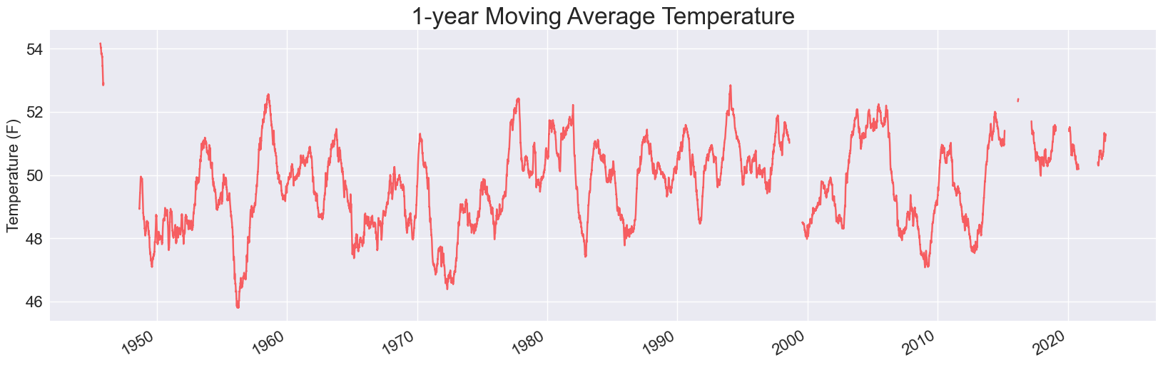
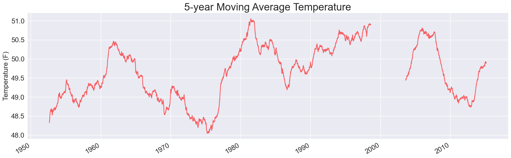
Each of these is missing some data. When we use pandas to read in data from a CSV file, it doesn’t skip over invalid rows. Instead, it fills those rows with NaN values, which is short for Not a Number. If we keep these values in the data set when running our analysis, they lead to holes in the visualizations.

Examining invalid data

Before deciding what to do with the invalid data, it’s a good idea to see how much data is missing or invalid.

Here’s a snippet that tells us how many data points were invalid:

...
# Extract data.
path = Path('wx_data/sitka_highs_1944_2023.csv')
dates, highs = get_data(path)
print(f"\nFound {len(highs):,} data points.")

num_invalid = highs.isna().sum()
print(f"There are {num_invalid} invalid readings.")

The method isna() checks if each item in a Series is NaN. The snippet highs.isna() returns a Series that’s the same length as highs, but only consists of the values True and False. Every NaN element in highs generates a True value, and every other element generates a False value in the resulting Series.

Here’s what the resulting Series looks like:

0       False
1       False
2       False
...
456     True
...
28092   False

In Python, int(True) returns 1. Chaining sum() on a sequence of Boolean values becomes a nice way to count how many True values there are in a sequence.

All that to say, highs.isna().sum() counts the number of invalid readings in highs:

Found 28,093 data points.
There are 42 invalid readings.

Since we’re primarily interested in the 30-year timeframe, we can safely ignore 42 invalid readings. These invalid readings will have a negligible impact on an average of 30 * 365 readings, at least in this exploratory work.

Ignoring invalid data

pandas provides a straightforward way to drop invalid data from a DataFrame. The df.dropna() method drops any invalid rows from a DataFrame.

So, all we need to do is add one line to the get_data() function to generate clean plots:

def get_data(path):
    """Extract data from file."""
    df = pd.read_csv(path)
    df['DATE'] = pd.to_datetime(df['DATE'])

    # Drop invalid readings.
    df.dropna(inplace=True)
    
    return df['DATE'], df['TMAX']

The inplace=True argument tells pandas to modify the existing DataFrame, rather than returning a new DataFrame without the invalid data.2

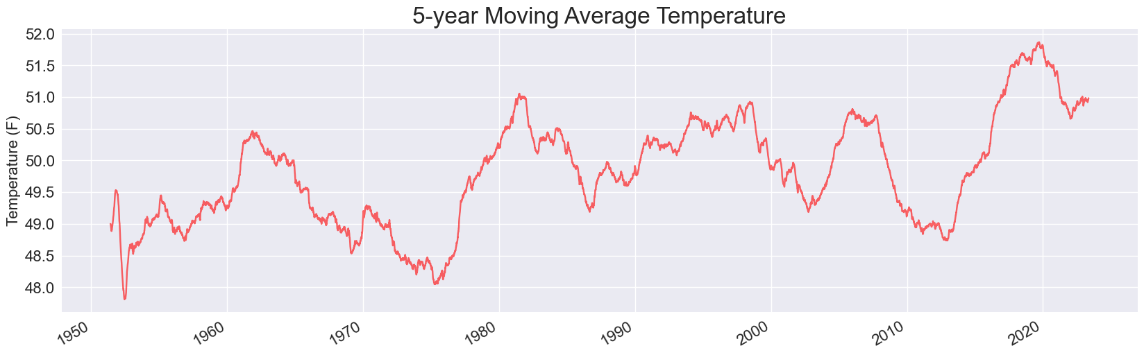
Adding this one line fixes the hole in all the plots. Here’s the 5-year plot:

And here’s the updated plot for a 30-year moving average:

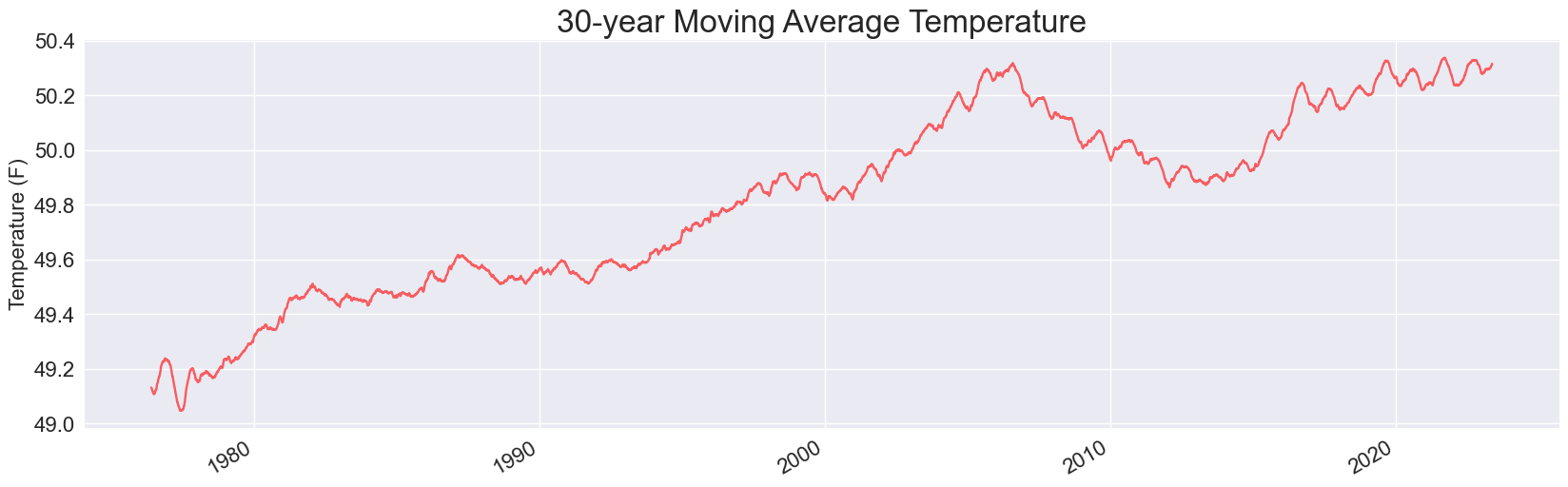
It looks like the drop in the early 2010s has reversed, and Sitka’s 30-year average temperature has just about matched its all-time high.

Looking at performance

This program runs plenty fast, but let’s profile a version of this code that generates the 30-year plot, to see how it compares to the standard library approach:

$ python -m cProfile -s cumtime high_temp_trends_30_yr.py

Found 28,051 data points.
         1501721 function calls (1474345 primitive calls) in 1.608 seconds

   Ordered by: cumulative time

   ncalls  tottime  percall  cumtime  percall filename:lineno(function)
       84    0.002    0.000    1.792    0.021 __init__.py:1(<module>)
    586/1    0.006    0.000    1.609    1.609 {built-in method builtins.exec}
        1    0.000    0.000    1.609    1.609 high_temp...30_yr.py:1(<module>)
   695/10    0.004    0.000    1.023    0.102 <frozen...

Even with more data points, there are fewer function calls. That makes sense, because we’re using pandas functions and methods in place of blocks of standard library code.

Without profiling, the 30-year program takes 1.1s to run, and the program that generates the full set of five plots takes only 2.2s.

Conclusions

While you can go a long way just using what’s in the Python standard library, it’s well worth your time to learn the basics of pandas if you’re going to be working with data on a regular basis. You can do more with less code, your code will be more readable, and it should run efficiently as well.

If your code starts to run slower than you like, make sure you profile it. Not everything in third-party libraries is better and faster, and a good profiling habit will help you identify the situations where third party code is not more efficient.

Resources

You can find the code files from this post in the mostly_python GitHub repository.

pandas documentation

If you’d like to look at some pandas documentation, here are a few good places to start:

• Visit the pandas homepage, and just start exploring.
• Read the overview. Many people skip this kind of documentation, and head straight for the more technical pages. But reading a page like this will help everything else you read about pandas make more sense.
• Skim the Series reference page.
• Skim the DataFrame reference page.
• Look at the Getting started articles, especially What kind of data does pandas handle?