The importance of profiling

When I first started using Python for data exploration, I didn’t know all that much about the scientific Python ecosystem. I used some plotting libraries, but I was unfamiliar with most of the data analysis tools. Many of the tools that we take for granted today were relatively new then as well.1 As a result, I did most of my analysis work using only the standard library. With a reasonable understanding of how to structure code, and how to use a profiler to guide optimization work, this approach worked well for a long time.

This post is the first of a two-part miniseries. In this post we’ll use just the standard library and Matplotlib to explore a local dataset. We’ll run a profiler, and sprinkle in a little NumPy to vastly improve the project’s performance. In the next post we’ll replace most of the standard library code with more concise pandas workflows. The code will be much shorter after that revision.

I still think there’s value in sharing code that primarily uses the standard library. Starting there gives you a much better understanding of what these newer tools are doing for us, and what optimizations have been made in their inner workings.

Don’t worry if you don’t follow all of the details of the data analysis work below. The main point about profiling and optimization will be clear, even if you don’t fully understand all of the code in the example. Feel free to skim everything until the “NumPy to the rescue” section.

Extracting climate patterns from weather data

You’ve probably heard it said that climate is different than weather. To focus on climate you need to get past short-term changes in weather and look at long-term trends. One simple way to do this is by using averages over large amounts of data.

I live in southeast Alaska, and reliable daily temperature data extends back to the 1940s. For this analysis, we’ll look at the daily high temperatures over a ~70 year period. The data set is here, and I’ve also included instructions for how to download your own data from the same source.2

Here’s a quick look at the data file:

# sitka_highs_1944_2012.csv

"STATION","DATE","TMAX"
"USW00025333","1944-09-01","59"
"USW00025333","1944-09-02","58"
"USW00025333","1944-09-03","64"
...
"USW00025333","2012-01-22","37"

The dataset goes from September 1, 1944 through January 22, 2012. It has three columns, which include the weather station name, the date of the reading, and the daily high temperature for that date.

Extracting data

Let’s extract the data from this file:

# high_temp_trends.py

from pathlib import Path
import csv
from datetime import datetime

def get_data(path):
    """Extract dates and high temperatures."""
    lines = path.read_text().splitlines()
    reader = csv.reader(lines)
    header_row = next(reader)

    dates, highs = [], []
    for row in reader:
        try:
            high = int(row[2])
            highs.append(high)
            current_date = datetime.strptime(row[1], '%Y-%m-%d')
            dates.append(current_date)
        except ValueError:
            print(row)

    return dates, highs

# Extract data.
path = Path('wx_data/sitka_highs_1944_2012.csv')
dates, highs = get_data(path)
print(f"\nFound {len(highs):,} data points.")

We write a function called get_data() to extract the data. We do this partly because encapsulating code in functions is a good idea in general, but also so that we’ll be able to use cProfile to identify any bottlenecks that come up.

In get_data(), we parse the CSV file and load any valid high-temperature data. Libraries like pandas automate a lot of what you see here, but it’s interesting to see how to do this using the standard library as well. Basically, we break the file into individual lines and create a csv.reader() object. We then look at every row in the file, and try to extract a high temperature, which is in the third column (index 2). We use a try-except block, because there could easily be some missing or corrupt data in a dataset this large. This function returns a list of dates and a corresponding list of high temperatures.

Here’s the output:

$ time python high_temp_trends.py
['USW00025333', '1945-12-01', '']
['USW00025333', '1945-12-02', '']
['USW00025333', '1945-12-03', '']
...
['USW00025333', '1945-12-31', '']
['USW00025333', '1998-08-11', '']

Found 23,941 data points.
python high_temp_trends.py  0.15s user 0.01s system 94% cpu 0.172 total

There are almost 24,000 valid data points. It looks like the weather station was not operational for a month in 1945, and one day in 1998. We also note that extracting the data took less than 0.2s, so we probably won’t need to optimize the data extraction part of this project.

Visualizing data

Before going any further, let’s see what this data looks like:

# high_temp_trends_visual.py

from pathlib import Path
import csv
from datetime import datetime

import matplotlib.pyplot as plt

def get_data(path):
    """Extract dates and high temperatures."""
    ...

def plot_data(dates, temps, title,
        filename="output/high_temps.png"):
    """Plot daily temperature data."""
    plt.style.use('seaborn-v0_8')
    fig, ax = plt.subplots(figsize=(20, 6))

    ax.plot(dates, temps, color='red', alpha=0.6)

    # Format plot.
    ax.set_title(title, fontsize=24)
    ax.set_xlabel('', fontsize=16)
    fig.autofmt_xdate()
    ax.set_ylabel("Temperature (F)", fontsize=16)
    ax.tick_params(labelsize=16)

    plt.savefig(filename, bbox_inches="tight")

# Extract data.
...

# Plot the data.
title = "Daily High Temperatures"
plot_data(dates, highs, title)

The function plot_data() accepts a sequence of dates and a sequence of temperatures, a title, and a filename. I’m saving the plot file instead of opening it in a viewer, so I can continue to time the overall execution time without measuring the time I’m looking at a plot viewer.

Here’s what this data looks like:

This data is much too noisy to see any long-term climate trends. We can see the missing month of data early in the dataset. It looks like there were some winters around 1960 that were warmer overall than others. But beyond that it’s hard to spot meaningful trends.

Analyzing the data

We want to look at long-term trends in the temperature data, and get rid of the daily fluctuations in high temperatures. We may want to get rid of the monthly and even annual fluctuations, but we’ll come back to that in a bit.

Moving averages

To look beyond daily fluctuations, we’ll calculate a moving average for every day. If you’re not familiar with moving averages, consider any single day in the dataset. Instead of asking what the high temperature was that day, which varies wildly, we’d like to know what the average high temperature was for the previous 30 days.

Here’s a function that returns a set of 30-day moving averages:

def get_averages(temps):
    """Calculate 30-day moving average over the entire dataset."""
    averages = []
    for index in range(30, len(temps)):
        temps_slice = temps[index-30:index]
        mean = statistics.mean(temps_slice)
        averages.append(mean)

    return averages

The function get_averages() needs a sequence of temperatures to analyze. We define an empty list that we’ll store the moving averages in. We can’t loop over the entire list of temperatures, because we can’t calculate 30-day averages until we have at least 30 days worth of data. We’re also going to be repeatedly looking at slices of data, so we’ll loop over the indexes that we’re interested in instead of the actual items.

The first temperature we want to look at is at index 30, and then we want to iterate through the entire remainder of the list. So, we loop over every index in the expression range(30, len(temps)).  In the loop, we want to look at the previous 30 measurements. Thinking about it from the perspective of the current date being examined, we want to iterate from “30 days ago through today”. That corresponds to the slice temps[index-30:index], which you might read as temps[30 days ago through today].

Once we have that slice, we take the average temperature over the last 30 days, and append it to the list averages. When we’ve finished analyzing the entire dataset, we return the list of averages.

Here’s the full program, with a generalized version of this function:

# high_temp_trends_30_day.py

from pathlib import Path
import csv, statistics
from datetime import datetime

import matplotlib.pyplot as plt

def get_data(path):
    ...

def get_averages(temps, timespan):
    # Calc moving averages over the entire dataset.
    avgs = []
    for index in range(timespan, len(temps)):
        temps_slice = temps[index-timespan:index]
        mean = statistics.mean(temps_slice)
        avgs.append(mean)

    return avgs

def plot_data(dates, temps, title, filename="high_temps.png"):
    ...

# Extract data.
...

# Analyze data.
timespan = 30
avgs = get_averages(highs, timespan=timespan)

# Plot the data.
title = f"{timespan}-day Moving Average Temperature"
relevant_dates = dates[timespan:]
plot_data(relevant_dates, avgs, title)

The main difference in this version of the function is the addition of a timespan parameter, which will let us work with moving averages of any duration.

When we plot the data, we define a timespan, customize the title, and make sure we choose the set of dates that correspond to what we’ll get back from get_averages().

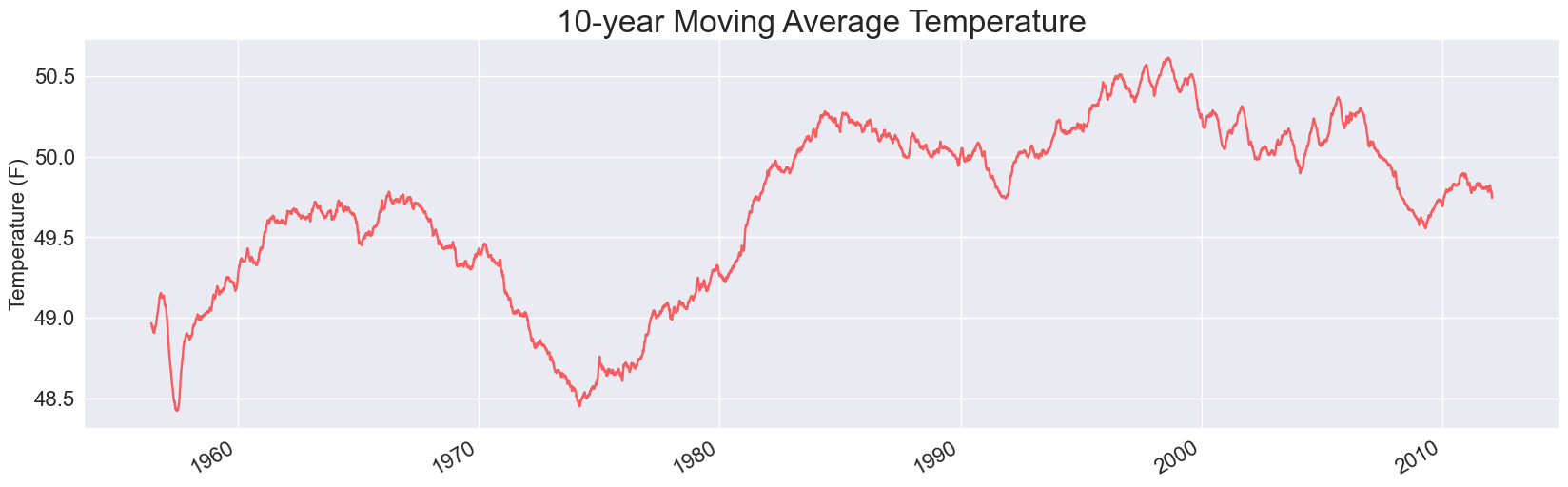
Here’s the resulting plot:

This is visibly less noisy; we’ve removed the daily fluctuations from the overall plot line. We can even start to notice some long term trends. I notice several winters before 1970 where the 30-day average high dips below 30F, but none since then. In fact, it looks like no winter since ~1985 has a 30-day average high temperate below freezing. (It would be interesting to run this same analysis for low temperatures.)

I’ll also note that this still takes just over a second, so we haven’t hit any significant bottlenecks yet.

Exploring different timespans

We don’t need to write any more code to explore this data. We can modify the value of timespan, and see how much it smooths out the data. Here’s a moving one-year average (timespan=365), which I would expect to smooth out the monthly variations:

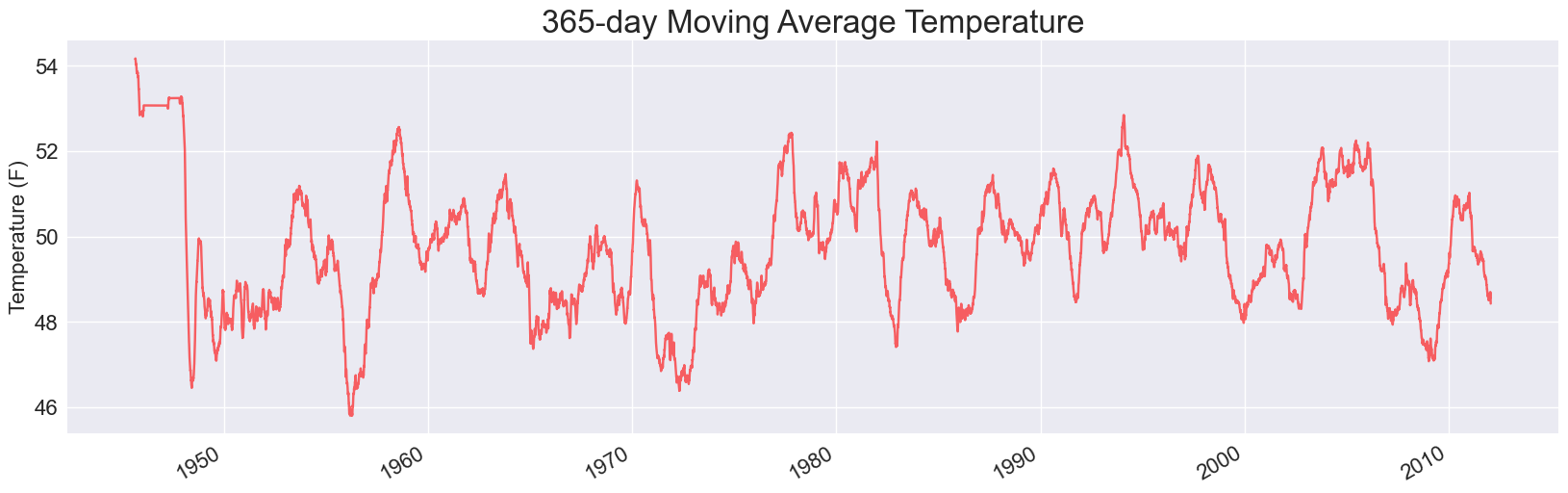
This is much different. The last plot has highs corresponding to average summer temperatures, and lows corresponding to average winter temperatures. When you increase the timespan to a full year, you get rid of the seasonal variations and start to see only yearly fluctuations. Note that the y-axis range on the last graph was about 20 degrees through 70 degrees; on this chart the range only goes from about 44 degrees to 56 degrees. Note that this analysis took almost 3 seconds to run; as the timespans get longer there’s more work to do when generating the averages.

Here are the plots for 5, 10, and 30-year timespans. The only change I’ve made to the code is to generate a title reflecting years rather than days:

This is quite interesting to see, if you haven’t run this kind of analysis before. In the 30-year average, which should smooth out all daily, seasonal, and annual fluctuations, this region’s daily high temperature increased by about one degree Fahrenheit between 1976 and 2006. It’s dropped about three-tenths of a degree since then.

But, there’s a problem with our code that’s becoming apparent. The 5-year plot took 8.3s to run, the 10-year plot took 14.4s, and the 30-year plot took 27s! If we want continue exploring data—either different timespans, or different kinds of temperature, or looking at a variety of locations—we’ll probably want to make our code more efficient if at all possible.

Let’s profile the code, and then see how NumPy can help.

Profiling

My guess before we run the profiler is that the bulk of the slowdown is happening inside get_averages().3 We’re not changing how the data is extracted, and we can still see in the terminal that the summary about extracting the data shows up almost immediately after running the program. The plots have less data for longer timespans, so I’m pretty sure the plotting code is not the issue.

Here’s the output of running the 30-year version of this file using cProfile:

$ python -m cProfile -s cumtime high_temp_trends_30_yr.py
...
Found 23,941 data points.
         429192644 function calls (429167718 primitive calls) in 138.656 seconds

   Ordered by: cumulative time

   ncalls  tottime  percall  cumtime  percall filename:lineno(function)
    289/1    0.003    0.000  138.656  138.656 {built-in...builtins.exec}
        1    0.000    0.000  138.656  138.656 h...yr.py:1(<module>)
        1    0.276    0.276  136.926  136.926 h...yr.py:25(get_averages)
    12991    0.027    0.000  136.648    0.011 statistics.py:414(mean)
    12991   73.653    0.006  136.513    0.011 statistics.py:154(_sum)
142251450   36.825    0.000   49.917    0.000 statistics.py:287(_exact_ratio)
142251450   13.091    0.000   13.091    0.000 {method 'as_integer_ratio' of 'int' objects}
142349255   12.783    0.000   12.783    0.000 {method 'get' of 'dict' objects}
       32    0.002    0.000    0.929    0.029 __init__.py:1(<module>)
      ...

This shows why the code is taking so long to run. There were 23,941 data points, but it took almost 430 million function calls to complete the analysis. Almost the entire execution time is spent in get_averages(). Most of that time is spent running code from the statistics.py module: mean(), _sum(), and _exact_ratio(). There are three calls here that are made over 140 million times each. It took over two minutes to profile this code (139 seconds).

Clearly, our optimization work needs to focus on the get_averages() function, and it should focus on the call to statistics.mean().

NumPy to the rescue

Let’s take another look at how get_averages() is currently implemented:

def get_averages(temps, timespan):
    # Calc moving averages over the entire dataset.
    avgs = []
    for index in range(timespan, len(temps)):
        temps_slice = temps[index-timespan:index]
        mean = statistics.mean(temps_slice)
        avgs.append(mean)

Almost the entire execution time is spent in that one line involving the call to statistics.mean(). This is where profiling is so helpful. Without that specific information, there are a number of other places I might have been tempted to start my optimization efforts.

I know that NumPy has a number of more efficient data structures, but I also know it has implementations of many common numerical operations. It has a mean() function, so let’s use it. The numpy.mean() function operates on an array, or an array-like sequence. Basically, if you give numpy.mean() something that it can convert to an array, it should be able to compute the mean for you.

We add a call to import numpy as np at the top of the file, and the call to statistics.mean() is replaced by a call to np.mean():

def get_averages(temps, timespan):
    # Calc moving averages over the entire dataset.
    avgs = []
    for index in range(timespan, len(temps)):
        temps_slice = temps[index-timespan:index]
        mean = np.mean(temps_slice)
        avgs.append(mean)

Here’s the profiling output, with that one-line change:

$ python -m cProfile -s cumtime high_temp_trends_30_yr_np_mean.py
...
Found 23,941 data points.
         2112979 function calls (2088080 primitive calls) in 7.857 seconds

   Ordered by: cumulative time

   ncalls  tottime  percall  cumtime  percall filename:lineno(function)
    288/1    0.003    0.000    7.858    7.858 {built-in method builtins.exec}
        1    0.000    0.000    7.858    7.858 h...yr_np_mean.py:1(<module>)
        1    0.257    0.257    6.129    6.129 h...yr_np_mean.py:26(get_averages)
17730/16480    0.015    0.000    5.905    0.000 {built-in method numpy.core._multiarray_umath.implement_array_function}
    12991    0.012    0.000    5.871    0.000 <__array_function__ internals>:177(mean)
    12991    0.043    0.000    5.846    0.000 fromnumeric.py:3345(mean)
    12991    0.049    0.000    5.803    0.000 _methods.py:164(_mean)
    16039    5.589    0.000    5.589    0.000 {built-in method numpy.asanyarray}
       32    0.002    0.000    0.930    0.029 __init__.py:1(<module>)

Operating on the same number of data points, there are far fewer function calls required to complete the analysis. We’ve dropped from almost 430 million function calls to just over 2 million calls. I believe the correct interpretation of this is that NumPy has moved most of the work to lower-level, highly optimized routines that don’t have nearly as much overhead as the mean() function in the Python standard library.

This profiling run took just under 8 seconds. Without profiling, the overall execution time for our program has dropped from about 27 seconds to about 7 seconds.

Going even faster

A program that takes 7 seconds to run is still going to get annoying, especially if there’s a straightforward way to speed it up. NumPy arrays are special sequences that are optimized for efficiency for many operations. There are some restrictions; they can only contain data of a single type, and you have to decide ahead of time how many elements they will contain.

Currently, we’re sending get_averages() a list of high temperatures to analyze. The function then iterates over this list repeatedly, taking many slices of that list as it calculates the moving averages. If we can do all of that work with an array, we might see some additional efficiency.

NumPy arrays are more complicated to create from scratch than lists, but if you already have a list containing only one data type you can often convert it to an array. Here’s the block of code that calls get_averages(), for calculating a 30-year moving average:

timespan = 365*30
avgs = get_averages(highs, timespan=timespan)

Instead of passing the list highs to get_averages(), let’s first convert it to a NumPy array and pass that to get_averages():

timespan = 365*30
highs_array = np.array(highs)
avgs = get_averages(highs_array, timespan=timespan)

Here’s the profiling results for this small change:

$ python -m cProfile -s cumtime high_temp_trends_30_yr_np_array.py
...
Found 23,941 data points.
         2112980 function calls (2088081 primitive calls) in 2.006 seconds

   Ordered by: cumulative time

   ncalls  tottime  percall  cumtime  percall filename:lineno(function)
    288/1    0.003    0.000    2.006    2.006 {built-in method builtins.exec}
        1    0.000    0.000    2.006    2.006 h...yr_np_array.py:1(<module>)
       32    0.001    0.000    0.921    0.029 __init__.py:1(<module>)

There’s one more function call than the last run, the call to np.array(). But this profiling run takes just over 2 seconds. All that work manipulating Python lists and slices has been moved to lower-level routines. A whole bunch of overhead is eliminated. Without profiling, this code has dropped to just 1.2 seconds for loading, analyzing, and plotting the data.

With just three lines of code and an additional import statement, we’ve dropped from 27 seconds to 1 second. That is impressive.

One more thing

I took a moment to automate the generation of plots with different timespans. A file that automatically generates plots for 1, 3, 5, 10, and 30-year timespans takes about 56 seconds to run using just lists. With the NumPy optimizations we found above, the same five plots are generated in just over 3 seconds. Profiling this shows that most of the program’s execution time is now spent in plot_data(). We’ve eliminated analysis as the bottleneck in this program!

Conclusions

If you’re doing exploratory data analysis work on a regular basis, it’s well worth your while to learn the modern Python data science stack instead of relying on the standard library. However, it’s good to see how this work can be done with a simpler set of tools:

• You learn a lot about core data structures in Python.
• When you start to use more specific tools, you have a better understanding of what those tools are doing for you.
• You learn a lot about profiling and optimization.
• You can still get meaningful work done in situations where you can’t install larger third party packages.

There’s no doubt about it, the Python data science toolset is incredibly powerful, and you should certainly be using it. But not every tool will magically make your code run fast, and it’s not always obvious what these tools are doing on your behalf. In these situations, a clear understanding of core data structures and workflows provides a strong foundation for figuring out how to use the more advanced tools in the most effective and appropriate ways.

Standard library functions, and functions in well-established third party packages, are almost always faster than functions you write yourself. Many of these functions have been optimized over the years by people with specialized knowledge. But sometimes library code is slower than code that you can write yourself. Maybe the library has to handle a wider range of use cases; maybe there’s another goal or constraint you're not aware of; or maybe you’re working with a seldom-used part of the library that hasn't been optimized in a long time. Profiling cuts through all these possibilities, and shows us exactly what to focus on.

In the next post we’ll repeat this entire process using a modern toolset. We’ll look at how this affects the simplicity of the code, as well as its performance throughout the development process. We’ll also update the dataset to extend through this year.

Resources

You can find the code files from this post in the mostly_python GitHub repository.